3. Usage
In this section, we provide a step-by-step guide with an example in which you can deploy an AI Agent to trigger Service Assurance scaling actions based on a common AI use case: pattern recognition in images. In our specific case we will scale-in/out VNF instances based on recognising traffic jam situations using real pictures from a motorway.
After this example, we also provide the ‘Deploying my own AI Agent’ section, where you can also see how to deploy your AI-Agents to build-up your specific AI applications based on OSM.
3.1. Quick Start: VNF scaling based on road-traffic images recognition.
This example is based on the usage of a Convolutional Neural Network (CNN) to classify images taken through a public road traffic control camera available through the following URL: http://www.dgt.es/es/el-trafico/camaras-de-trafico/madrid/a-2/pk-003.290-c.shtml. The objective is to trigger scaling actions of a VNF (scale-in and out) depending on the road traffic density in one of the directions of the motorway (scale-out when the traffic density is high, and scale-in otherwise); for instance:
Of course, the neural network is expected to be insensitive to slight variations in framing (the camera moves at times) and lighting (providing a correct response regardless of whether the day is sunny, cloudy, at night…). To avoid over-complicating the explanation, we will not go into details of the neural network itself.
The following figure shows the set-up for implementing this exercise:
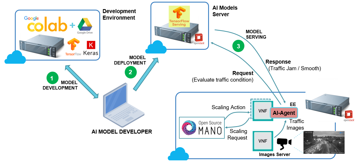
Road-traffic example set-up
As we see, the AI Model developer (you) will use a development environment based in Google Colab to develop and train the AI Model (the CNN), leveraging on the well-known AI framework TensorFlow and Keras (the Python Machine Learning API). Don’t panic: we’ll provide you here the source code and the step-by-step procedure for implementing this.
Once the AI Model is trained, it will be deployed on the AI-Models Server (step 2 in the figure). After that, we will deploy a VNF on OSM with the AI-Agent attached. The AI-Agent will query the AI-Model with the images from the Images Server (this is another VNF that simply provides the road-traffic images). Based on the AI Models Server response the VNF will be scaled-in or out.
Pre-requisites
Before continuing reading, make sure you have the following:
An OSM Release NINE (or later) installation (if you need it, you can find the installation procedure right here: Install OSM based on k8s ).
The AI Models Server to deploy the AI model. For this example we will use TensorFlow Serving for implementing the AI Models Server (however, other AI frameworks could be used as well). You can find the TensorFlow Serving installation procedure in Annex 1.
Step-by-step procedure
A. Develop and Train the AI Model
As previously mentioned, we will rely on Google Colab framework for the development of the AI Model (see figure below). In this framework we will use the TensorFlow and Keras to develop the AI Model (Google Colab relies on Google Drive for the data storage).
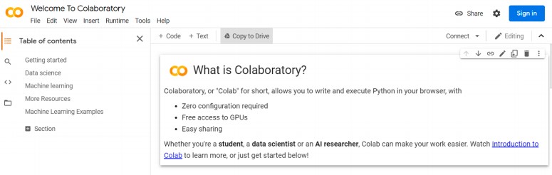
To start working with Google Colab you need first to authenticate yourself with a Google account. Once inside, click on “File -> New Notebook”. In this way, a cell for the development of the python code will open:
After that, you can paste in this cell the following code, which is used to perform the training of the Convolutional Neural Network described above (as you can see many comments have been introduced to help you understand the code):
"""
Import the required libraries
"""
import sys
import os
from tensorflow.python.keras.preprocessing.image import ImageDataGenerator
from tensorflow.keras import optimizers
from tensorflow.python.keras.models import Sequential
from tensorflow.python.keras.layers import Dropout, Flatten, Dense, Activation
from tensorflow.python.keras.layers import Convolution2D, MaxPooling2D
from tensorflow.python.keras import backend as K

"""
Init a new keras session and link to Google Drive, which is what we use as file system.
Images are expected to be stored in the 'My Drive/Colab Notebooks/TrafficData' directory, under
the 'Training' and 'Validation' sub-folders (training and validation images respectively).
"""
K.clear_session()
google = !if [ -d 'GDrive/' ]; then echo "1" ; else echo "0"; fi
if (google[0] is '0' ):
from google.colab import drive
drive.mount('/content/GDrive/')
!if [ -d 'GDrive/' ]; then echo "Connection to Google drive successful" ; \
else echo "Error to connect to Google drive"; fi

data_path = '/content/GDrive/My Drive/Colab Notebooks/TrafficData'
data_training = data_path + '/Training'
data_validation = data_path + '/Validation'

"""
Params
"""
#Size to which we are going to cut our images (Original: 853 x 480 pixels)
image_width, image_height = 100, 100

#Times we're going to iterate over the data set during the training stage
epochs = 25

#batch size = images to process at each step
batch_size = 5

#Number of filters to apply in each convolution. After Conv1 our image will have
#depth=64; after Conv2 the image will have depth=128.
filtConv1 = 64
filtConv2 = 128

#Size of the filters to be used in convolutions. Coordinates represent height and length
#of the filter.
size_filt1 = (3, 3)
size_filt2 = (2, 2)

#Size of the filter to be used during the MaxPooling stage
size_pool = (2, 2)

#We need to classify 2 different classes: high and low traffic density
classes = 2

"""
Images pre-processing (before presenting them to the neural net)
"""
#Create image data generators for the images in the training and the validation sets.
#In both cases RGB values are normalized from 0 to 1 (instead from 0 to 255)
training_datagen = ImageDataGenerator(rescale=1./255)
test_datagen = ImageDataGenerator(rescale=1./255)

#Now let's generate the images that will be actually used for training the net. The following
#'flow_from_directory' commands do the following: enter the corresponding directory (training
#or #validation), open all folders and process the images with a specific height and length.
#'categorical' means that the classification will be done by categories (fluid or dense
#traffic in our case).
training_generator = training_datagen.flow_from_directory(
    data_training,
    target_size=(image_height, image_width),
    batch_size=batch_size,
    class_mode='categorical')

validation_generator = test_datagen.flow_from_directory(
    data_validation,
    target_size=(image_height, image_width),
    batch_size=batch_size,
    class_mode='categorical')

#Print-out all the declared classes (useful for the classification program once the CNN is trained)
print('Classes: ', training_generator.class_indices)

"""
Create the Convolutional Neural Network
"""
cnn = Sequential() #Secuencial Net (stacked layers model)

#Execute the first stage of convolution and pooling with the parameters defined above.
cnn.add(Convolution2D(filtConv1,
              size_filt1,
              padding ="same",
              input_shape=(image_width, image_height, 3),
              activation='relu'))
cnn.add(MaxPooling2D(pool_size=size_pool))

#Second stage of convolution and pooling (input-shape not needed here)
cnn.add(Convolution2D(filtConv2,  size_filt2, padding ="same"))
cnn.add(MaxPooling2D(pool_size=size_pool))

#We flatten the images now to a single dimension (they are small and deep now)
cnn.add(Flatten())

#We add here two consecutive 'regular' (non-convolutional) layers with 256 and 16 nodes to
#process the flatten input generated in the previous stage
cnn.add(Dense(256, activation='relu'))
cnn.add(Dense(16, activation='relu'))

#In the previous dense layers we 'turn off' 25% of the neurons randomly at each step during
#the training. This is done to minimize over-fitting problems.
cnn.add(Dropout(0.25))

#Output layer. Number of neurons equal to the number of classes. Activation type
#'softmax' (each neuron identifies each of the classes).
cnn.add(Dense(classes, activation='softmax'))

#We now compile the CNN. The compiling parameters are:
# -loss     : represents the loss function, i.e., the way the algorithm sees how well or badly
#             it is doing). In this case we use the 'categorical crossentropy' function
# -optimizer: type 'Adam', which is an advanced version of the backpropagation algorithms
# -metric   : measures how well the network is learning.
cnn.compile(loss='categorical_crossentropy', optimizer='adam', metrics=['accuracy'])

"""
Training stage
"""

#Now we compute the steps for the training and validation stages. This way we automatically
#get the necessary steps according to the number of images supplied (the steps represent the
#number of times the information is processed in each of the epochs we have defined; at the
#end of each training epoch we run the 'n' validation steps that are computed here).
t_steps = training_generator.n // training_generator.batch_size
v_steps = validation_generator.n // validation_generator.batch_size
print('training_steps  : ', t_steps)
print('validation_steps: ', v_steps)

#Here the training itself. What we say here is that we are going to train our CNN with the
#training images and during the defined epochs. We also say which are the validation images
#and the validation steps. In our specific case what the network will do is to run 'steps'
#steps in each of the epochs; when each epoch ends it will run 'validation_steps' validation
#steps and then it will move on to the next epoch.
cnn.fit(
    training_generator,
    steps_per_epoch=t_steps,
    epochs=epochs,
    validation_data=validation_generator,
    validation_steps=v_steps)

"""
Exporting the trained model
"""
#When the training is finished we save the result in a couple of 'h5' files (one for the
#topology, and another one for the weights).
target_dir = data_path + '/ResultingModel'
if not os.path.exists(target_dir):
    os.mkdir(target_dir)
cnn.save(data_path + '/ResultingModel/traffic-model-topology.h5')
cnn.save_weights(data_path + '/ResultingModel/traffic-model-weigths.h5')
As you can see, the program expects to find the training images in Google Drive. The images used to train and verify the model are contained in three zip files, with the following directories:
Training: Training images (two sets, with images in traffic jam situations and with flowing traffic).
Validation: Validation images during training (same two sets).
Production Images: Images used after training and validation to evaluate the classification capacity of the model (images here were used neither during training nor during validation, so they are useful for verifying the performance of the network once trained).
All these images are available: here (see ProductionImages.zip, TrainingImages.zip and ValidationImages.zip).
In each of the folders (Training, Validation and Production) there are images with different lighting conditions (day, night, cloudy days, sunny days, rainy days…) and with different framing conditions (there are small variations in zoom and the focus angle). The number of images in the Training, Validation and Production folders is the same for the two cases we want to classify (traffic jams and low traffic density).
The images should be located in Google Drive under the directory “/content/GDrive/My Drive/Colab Notebooks/TrafficData”, inside of it there should be two folders: “Training” (with the training images) and “Validation” (with the validation images). Therefore, before running the program it will be necessary to move the images provided in the repository.
To execute the code, click on the arrow-shaped button in the cell on its left-hand side. The first time you execute the program you will be asked for permission to access your Google Drive account (a link will appear on which you have to click to get a verification code). In Google Colabs, Google Drive is not only used to access the collection of images, but also to write the model data (topology and weights) once the neural network is trained.
The training process takes a while (few minutes typically). During the training the following output is shown:
As you can see 25 epochs of training are executed, with 27 steps on each one (the steps per epoch are automatically computed by the program). The ‘val_accuracy’ parameter represents how well the neural network classifies the images during the training. ‘1.0’ represents a 100% success rate. As we see the learning process starts with a 0.6 value (60%) which increases during the process until it reaches values close to 100% on average.
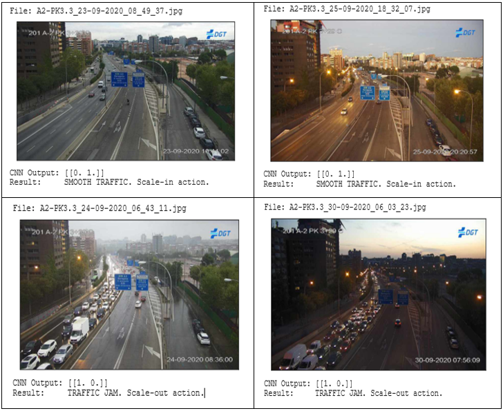
Once the training is finished you can execute the following program (also in a Google Colab cell) to evaluate the performance of the AI Model on the Production Images set:
import os
import numpy as np
from keras.preprocessing.image import load_img, img_to_array
from keras.models import load_model
import matplotlib.pyplot as plt
import matplotlib.image as mpimg

# Connect to Google Drive, which is where we have stored the images
google = !if [ -d 'GDrive/' ]; then echo "1" ; else echo "0"; fi
if (google[0] is '0' ):
    from google.colab import drive
    drive.mount('/content/GDrive/')
!if [ -d 'GDrive/' ]; then echo "Connection to Google drive successful" ; \
else echo "Error to connect to Google drive"; fi

files_path = '/content/GDrive/My Drive/Colab Notebooks/TrafficData/'

# Images size. Must match the values we set for the training process. The original size was
# 853x480 pixels, but we reduced to 100x100 during the training.
img_width, img_height = 100, 100

# Load Neural Network topology and weights (h5 files generated during the training)
topology = files_path + 'ResultingModel/traffic-model-topology.h5'
weights = files_path + 'ResultingModel/traffic-model-weigths.h5'
cnn = load_model(topology)
cnn.load_weights(weights)

# Function that receives the image and tell if there is a traffic jam (or not)
def predict(file):
  x = load_img(file, target_size=(img_width, img_height))
  x = img_to_array(x)
  x = np.expand_dims(x, axis=0)

  #This is where we invoke the CNN by passing the formatted image as a parameter. The result
  #is a two-dimensional array (because we had two neurons at the output layer).
  arr = cnn.predict(x)
  print('CNN Output:', arr)
  if np.argmax(arr[0]) == 0:
    print('Result:     TRAFFIC JAM. Scale-out action.')
  else:
    print('Result:     SMOOTH TRAFFIC. Scale-in action.')
  print('-------------------------------------------------')

# Check all images in the corresponding directory and print out the result (you can set the
# directory name to 'LowDensity' or 'HighDensity' to use images with low/high traffic density).
sourcedir = files_path + 'ProductionImages/LowDensity/'
print('>>>> Results for files in \''+ sourcedir + '\' directory:\n')
dir = os.listdir(sourcedir)
for f in dir:
  print('File: ' + f)
  img = mpimg.imread(sourcedir + f)
  imgplot = plt.imshow(img)
  imgplot.axes.get_xaxis().set_visible(False)
  imgplot.axes.get_yaxis().set_visible(False)
  plt.show()
  predict(sourcedir + f)
As you can see, the program uses the ‘h5’ files generated during the neural network training. It iterates over the images into the “ProductionImages/LowDensity” and “ProductionImages/HighDensity” directories (they should be also under the “/content/GDrive/My Drive/Colab Notebooks/TrafficData” directory in Google Drive) that of course need to be filled with the corresponding images of the “Production” zip file).
As previously mentioned, those images were not used during the training process, so we can evaluate how the network would respond to images that never processed before. In the set there are of course different kind of images, i.e., with different light conditions, framing, etc.
The program produces an output similar to the following one for all the images in the ProductionImages directory:
B. Deploy the AI Model on the AI Models Server
As we have seen, by running the network training program as described before the model is stored in a couple of h5 format files under the “TrafficData/ResultingModel” directory in Google Drive.
However, what we need is to have a model that can be deployed on the TensorFlow Serving instance (and that can be queried from the AI Agents deployed under the OSM scope).
The first step do this is to transform the h5 files into protobuf (PB) files, which are the files supported by the TensorFlow Serving platform (see here for more information about this format). To perform this conversion you can use the following code (you can execute it also as a separated Google Colab cell):
import tensorflow as tf
import tempfile
import os

MODEL_DIR = tempfile.gettempdir()
version = 1
export_path = os.path.join(MODEL_DIR, str(version))
print('export_path = {}\n'.format(export_path))

tf.keras.models.save_model(
    cnn,
    export_path,
    overwrite=True,
    include_optimizer=True,
    save_format=None,
    signatures=None,
    options=None
)

print('\nSaved model:')
!ls -l {export_path}

!zip -r /tmp/A2-traffic-model.zip /tmp/1

from google.colab import files
files.download('/tmp/A2-traffic-model.zip')
The execution takes a while. The output should be similar to this:
export_path = /tmp/1

INFO:tensorflow:Assets written to: /tmp/1/assets

Saved model:
total 188
drwxr-xr-x 2 root root   4096 Sep 28 10:37 assets
-rw-r--r-- 1 root root  17753 Sep 28 10:37 keras_metadata.pb
-rw-r--r-- 1 root root 163332 Sep 28 10:37 saved_model.pb
drwxr-xr-x 2 root root   4096 Sep 28 10:37 variables
  adding: tmp/1/ (stored 0%)
  adding: tmp/1/assets/ (stored 0%)
  adding: tmp/1/variables/ (stored 0%)
  adding: tmp/1/variables/variables.data-00000-of-00001 (deflated 5%)
  adding: tmp/1/variables/variables.index (deflated 65%)
  adding: tmp/1/keras_metadata.pb (deflated 91%)
  adding: tmp/1/saved_model.pb (deflated 87%)
As we see the code generates a zip file (A2-traffic-model.zip) with the AI model we have developed (network topology and weights) which can be now deployed on TensorFlow Serving. As we can see the model is stored in the ‘/tmp/1’ directory, where ‘1’ represents the version number we have assigned to the model (TensorFlow Serving supports the deployment of different versions of the same model). This zip file has to be downloaded from the ‘Google Colab’ environment to our local computer for its deployment on TensorFlow Serving. The steps to perform that deployment are as follows:
On the node you’ve TensorFlow Serving installed create the ‘A2-traffic-model’ directory under the ‘models’ directory (if you followed the procedure in Annex 1 to install TensorFlow Serving the path should be: ‘/home/ubuntu/serving/tensorflow_serving/tools/docker/tensorflow_serving_tutorial/model_volume/models/A2-traffic-model’).
Transfer the ‘A2-traffic-model.zip’ file from your local machine to the machine where we you have TensorFlow Serving installed. Place the file in the ‘models/A2-traffic-model’ directory created in the previous step:
$ scp A2-traffic-model.zip ubuntu@<tensorflow serving IP>:/home/ubuntu/serving/tensorflow_serving/tools/docker/tensorflow_serving_tutorial/model_volume/models/A2-traffic-model
    A2-traffic-model.zip  100% 222MB 3.6MB/s
Unzip the zip file we just transferred:
$ ssh ubuntu@<tensorflow serving IP>
$ cd ~/serving/tensorflow_serving/tools/docker/tensorflow_serving_tutorial/model_volume/models/A2-traffic-model
$ unzip A2-traffic-model.zip
    Archive: A2-traffic-model.zip
    creating: tmp/1/
    creating: tmp/1/variables/
    inflating: tmp/1/variables/variables.data-00000-of-00001
    inflating: tmp/1/variables/variables.index
    inflating: tmp/1/saved_model.pb
    creating: tmp/1/assets/
Declare the new model in the ‘models.config’ file including the following entry (path ‘/home/ubuntu/serving/tensorflow_serving/tools/docker/tensorflow_serving_tutorial/model_volume/configs’):
model_config_list: {
    config: {
        name: "A2-traffic-model",
        base_path: "/home/models/A2-traffics-model/tmp
        model_platform: "tensorflow"
        model_version_policy: {
            all: {}
        }
    }
}
Reload the server executing the following:
$ sudo docker run -it -p 8500:8500 -p 8501:8501 -v
   /home/ubuntu/serving/tensorflow_serving/tools/docker/tensorflow_serving_tutorial/mod
   el_volume/:/home/ test-tensorflow-serving
$ tensorflow_model_server --port=8500 --rest_api_port=8501 --model_config_file=/home/configs/models.conf
Once all the steps have been completed, you can check that the model has been actually deployed by accessing the model metadata from a web browser using the following URL: http://TensorFlowServingIP:8501/v1/models/A2-traffic-model/metadata.
After checking the model is accessible, you can also make some requests from your CLI passing the images to the model as parameters (this is just for testing the behaviour of the model you’ve deployed on TensorFlow Serving). You can create a small Python program to do this with the following source code:
import sys
import json
import requests
import nsvision as nv
print('Starting client...')
#Process provided arguments (server IP and image file)
if len(sys.argv) != 3
    print('ERROR. Usage: A2-traffic-model_clienti.py <Server IP:PORT> <image file>')
    sys.exit(2)

print('Processing image: ', end=" ")
print(sys.argv[2])
#Create JSON for REST call for a specific image
image = nv.imread(sys.argv[2],resize=(100,100),normalize=True)
image = nv.expand_dims(image,axis=0)
data = json.dumps({"instances": image.tolist()})
headers = {"content-type": "application/json"}

#print('JSON:')
#print(headers)
#print(data)

#Get result from server
response = requests.post('http://'+sys.argv[1]+'/v1/models/A2-traffic-model:predict',
data=data, headers=headers)
print('JSON response:', end =" ")
print(response.json())
#Process the response and print out the result
result_node0 = round(response.json()['predictions'][0][0])
result_node1 = round(response.json()['predictions'][0][1])
if result_node0 == 1 and result_node1 == 0:
    print('Result: TRAFFIC JAM. Scale-in action.')
else:
    print('Result: SMOOTH TRAFFIC. Scale-out action.')
print('Done')
As you can see, the code works as a client that encodes the selected image in JSON and makes the requests to TensorFlow Serving to retrieve the result corresponding to the encoded image. Below a couple of execution examples in our environment:
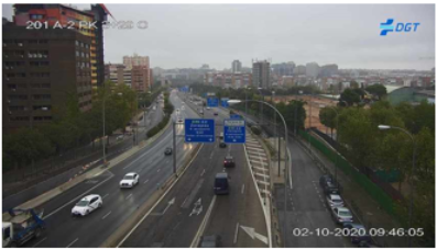
$ python3 A2-traffic-model_client.py 192.168.137.46:8501 Images/TrafficJam/A2-PK3.3_30-09-2020_08_16_09.jpg
Starting client...
Processing image: Images/TrafficJam/A2-PK3.3_30-09-2020_08_16_09.jpg
JSON response: {'predictions': [[0.992905319, 0.00709469151]]}
Result: TRAFFIC JAM. Scale-in action.
Done
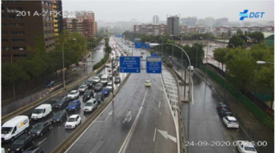
$ python3 A2-traffic-model_client.py 192.168.137.46:8501 Images/Smooth/A2-PK3.3_24-09-2020_11_52_56.jpg
Starting client...
Processing image: Images/Smooth/A2-PK3.3_24-09-2020_11_52_56.jpg
JSON response: {'predictions': [[3.50028534e-10, 1.0]]}
Result: SMOOTH TRAFFIC. Scale-out action.
Done
(images in these examples are in the “ProductionImages” directory previously mentioned).
C. Deploy the Monitoring Service
The Monitoring Service provides the required data to feed the AI Model hosted in the AI Models Server. In a real-life scenario this service would be in charge of collecting live traffic camera images, but in our example here we will deploy a basic Python script in a VM exposing a set of traffic images on a port that the AI Agent can reach via HTTP (this is done to avoid depending on external traffic cameras to execute our example).
To ease our testing the Monitoring Service is programmed to make possible to toggle between traffic jam and smooth traffic situations just by accessing a specific endpoint from a web browser (URL: ‘http://<MonitoringServiceIP>:3000/jam’). The way the service works is as follows: the service has access to two sets of images, being one set with traffic jam situations and another set with smooth traffic situations. Each time the endpoint is accessed from the web browser the service stops supplying photos from one set and starts supplying photos from the other set. This is used to force the service to deliver images of one type or another to facilitate our testing.
To deploy the Monitoring Service you can perform the following steps:
Create a python script in your preferred IDE with the following content, and name it as ‘app.py’:
import os
from flask import Flask, Response, request, abort, render_template_string, send_from_directory, jsonify
from PIL import Image
from io import StringIO
import random
import nsvision as nv
from waitress import serve
app = Flask(__name__)

jam = False

@app.route('/jam')
def change():
    global jam
    message = 'JAM enabled'
    if jam:
        jam = False
        message = 'JAM disabled'
    else:
        jam = True
    return message

@app.route('/')
def to_train():
    dir = 'normal'
    if jam:
        dir = 'jam'
    filename = random.choice(os.listdir('./Images/'+dir))
    print(filename)
    image = nv.imread('./Images/' + dir + '/' + filename, resize=(100, 100), normalize=True)
    image = nv.expand_dims(image, axis=0)

    return jsonify({"instances": image.tolist()}), 200

if __name__ == '__main__':
    serve(app, port= 3000)
- Prepare a dockerfile to deploy the monitoring service:
# set base image (host OS)
FROM python:3.8

# set the working directory in the container
WORKDIR /server

RUN pip install --upgrade pip
RUN pip install nsvision pillow flask waitress

COPY . /server

EXPOSE 3000
CMD [ "python", "app.py" ]
Include the collection of images to be exposed:
You can download the images set from here: (‘Images.zip’ file). If you want to change the images make sure the structure of this file is always as follows: .. code-block:
Images
    jam
    normal
app.py
dockerfile
Build the docker image:
docker build -t imageServer:latest .
The Monitoring Service has to be deployed as a docker image in a VM in the same VIM where OSM is running. To set-up the Monitoring Service in this way, you simply need to run the docker image generated earlier:
docker run -p 3000:3000 imageServer:latest
D. Prepare the AI Agent VNF and NS
Of course, instead of making manual requests to the AI Models Server from the command line, what we want is an AI Agent making requests and perform scaling actions based on the received responses. To do so we need to prepare a VNF with an embedded AI-Agent, and depoy that VNF as a Network Service in OSM.
To save you the work of having to do all this yourself for this demo we have already prepared a VNF and a NS which you can find here (‘ai-agents_ee_vnf.tar.gz’ and ‘ai-agents_ee_ns.tar.gz’ files).
Anyway, for the case you have to develop your own AI-Agents, we explain here how this VNF has been built.
As already mentioned in Section 1 (Scope) AI Agents are deployed using Helm Charts, so an important configuration file in the VNF package is the ‘values.yaml’ file. You can take a look to this file by decompressing the ‘ai-agents_ee_vnf.tar.gz’ file (using 7-zip, gunzip or another similar tool) and accessing under ‘ai-agents_ee_vnfhelm-chartseechartchartsai-agent’.
Note: You have to consider this file as something that is intimately linked to the VNF code and its functionality. If you develop another VNF with a different functionality than the one described here you will have to adjust the fields in this file as well (just as the source code of the VNF will also be different). Nevertheless we consider that this example can serve as a guide for your own developments.
** Pendiente: me gustaría poner esta nota anterior como un recuadro. Se puede? **
Here a sample of this file for your convenience:
The meaning of the different attributes in this file is as follows:
jobs. Pendiente. Decidme por favor que es esto.Podría haber más de un job?
name. Free text to designate the job.
image. This is to designate the images repository and its behaviour. Pendiente. Explicar más por favor. Tambien: ¿Qué significan los tres campos ‘repository’, ‘tag’ y ‘imagePullPolicy’? Explicadlo por favor.
schedule. The AI Agents makes periodic requests at regular intervals to the AI Models Server. This field indicates how often these requests are made. The same syntax is used as for the unix crontab command (see here).
failedJobsHistoryLimit. Pendiente. Qué Significa. Explicar please.
successfulJobsHistoryLimit. Pendiente. Qué Significa. Explicar please.
concurrencyPolicy. Pendiente. Qué Significa. Explicar please.
restartPolicy. Pendiente. Qué Significa. Explicar please.
env. Pendiente. Qué Significa. Explicar please.
config. Pendiente. Qué Significa. Explicar please.
predictions. This attribute is used to configure the different AI Models the AI Agent can interact to. In the example above two different models are configured (‘A2-traffic-model’ and ‘CPU-forecast-model’), with the corresponding parameters that are described below. Pendiente: Dudas: ¿un mismo AI Agent se puede conectar a la vez con más de un modelo? En ese caso ¿el schedule que configuramos arriba sería común para todos los modelos? ¿también las imágenes? ¿tiene sentido? Explicar por favor.
active. This is a boolean flag to activate/deactivate each configured model. For our example here the ‘A2-traffic-model’ should be set to ‘True’ (this is the AI model we’ve already deployed on the AI Models Server).
model/endpoint. This is the AI Models Server endpoint where our AI Model is served.
monitoring/endpoint. This is the Monitoring Server endpoint (the ancillary VNF serving the traffic images described in section C above).
threshold/function_name and logic. These parameters require a detailed explanation: The AI Agent has been designed to post the monitoring data to the configured endpoint, and will receive a JSON object formatted by Tensorflow Serving as:
{
    "predictions": [ [neu1, neu2] ]
}
Where ‘neu1’ and ‘neu2’ represent the values of the neurons pair in the output layer of the neural network. Considering this a traffic jam situation is identified when condition `x['predictions'][0][0] < x['predictions'][0][1]` is met. This information allow us to configure this Threshold section
using a lambda evaluator as shown above, i.e.:
threshold:
    function_name: evaluator
    logic: "evaluator = lambda x: False if (x['predictions'][0][0] < x['predictions'][0][1]) else True "
E. Run the demo
Once we have the descriptors for the VNF and the NS we can run the demo. You can follow the steps below to do so:
Onboard the VNF descriptor to OSM via OSM CLI or OSM UI. This is a regular procedure if you are familiar with OSM. Anyway you can refer to the OSM VNF Onboarding Guide.
Onboard the NS descriptor to OSM via OSM CLI or OSM UI. You can also refer to the OSM NS Onboarding guide here.
Instantiate the NS via OSM CLI or OSM UI. This is also a regular procedure in OSM. Anyway you can also refer to the OSM NS instantiation guide like in the previous steps.
Let some minutes go by and check that no scaling operations have been recorded for the VNF (considering that the monitoring service is exposing images with no traffic jam):
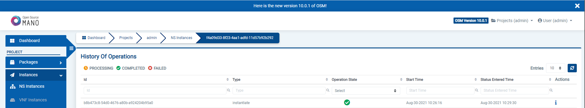
OSM UI with no scaling operations for the deployed NS
You can also check the AI-Agent traces. To do so first execute ‘kubectl get pods -n osm’ in the commands line to identify the K8s pod associated to the AI Agent; e.g.:
ubuntu@osm10:~$ kubectl get pods -n osm
NAME                                           READY   STATUS      RESTARTS   AGE
eechart-0093563749-ai-agent-1630482240-4cgvp   0/1     Completed   0          17s
grafana-755979fb8c-k6xld                       2/2     Running     0          34d
kafka-0                                        1/1     Running     0          34d
keystone-786dbb778d-qk8z5                      1/1     Running     0          34d
lcm-69d8d4fb5c-kmzd7                           1/1     Running     0          34d
modeloperator-77865c54-44ddm                   1/1     Running     0          34d
mon-7c966fccfb-22zqz                           1/1     Running     0          34d
mongodb-k8s-0                                  2/2     Running     0          34d
mongodb-k8s-operator-0                         1/1     Running     0          34d
mysql-0                                        1/1     Running     0          34d
nbi-6c8b6dffb4-rjd7g                           1/1     Running     0          34d
ng-ui-6d55c58954-wq7d8                         1/1     Running     0          34d
pol-66bff9db8c-nhhl5                           1/1     Running     0          34d
prometheus-0                                   1/1     Running     0          34d
ro-5d958cc7f9-cgzrl                            1/1     Running     0          34d
zookeeper-0                                    1/1     Running     0          34d
The K8s pod is the one with the ‘eechart’ prefix (‘eechart-0093563749-ai-agent-1630482240-4cgvp’ in this case).
Once you have the pod identifier you can access the traces as follows>
ubuntu@osm10:~$ kubectl logs -n osm eechart-0093563749-ai-agent-1630482240-4cgvp
{"asctime": "2021-09-01 07:44:15.074", "levelname": "INFO", "name": "utils", "message": "Checking Config:\n{'predictions': [{'active': False, 'monitoring': {'endpoint': 'http://192.168.137.34:4000'}, 'model': {'endpoint': 'http://192.168.137.46:8501/v1/models/CPU-forecast-model:predict'}, 'threshold': {'function_name': 'evaluator', 'logic': \"evaluator = lambda x: True if x['predictions'][0][0] >= 0.8 else False\"}}, {'active': True, 'monitoring': {'endpoint': 'http://192.168.137.34:3000'}, 'model': {'endpoint': 'http://192.168.137.46:8501/v1/models/A2-traffic-model:predict'}, 'threshold': {'function_name': 'evaluator', 'logic': \"evaluator = lambda x: False if (x['predictions'][0][0] < x['predictions'][0][1]) else True \"}}]}"}
{"asctime": "2021-09-01 07:44:15.094", "levelname": "INFO", "name": "osm_interface", "message": "VNFi info extracted from OSM: {'member-vnf-index-ref': 'VyOS Router', 'nsi_id': 'f3bf850f-6c47-42d0-bab4-7a3d3a1046d7', 'vdu-data': [{'vdu-id-ref': 'vyos-VM', 'ip-address': '192.168.137.43', 'name': 'aiagenttest-VyOS Router-vyos-VM-0'}], 'ns_name': 'aiagenttest', 'vnfs': ['648b8bb3-7f09-41ef-8a31-d632d1a90a8a'], 'project_id': '30ec57f1-4e48-43ce-a0f1-b136d66f9f67', 'scaling-group-descriptor': 'vyos-VM_vdu_autoscale'}"}
{"asctime": "2021-09-01 07:44:15.094", "levelname": "INFO", "name": "agent", "message": "OSM Data to run model evaluation: {'member-vnf-index-ref': 'VyOS Router', 'nsi_id': 'f3bf850f-6c47-42d0-bab4-7a3d3a1046d7', 'vdu-data': [{'vdu-id-ref': 'vyos-VM', 'ip-address': '192.168.137.43', 'name': 'aiagenttest-VyOS Router-vyos-VM-0'}], 'ns_name': 'aiagenttest', 'vnfs': ['648b8bb3-7f09-41ef-8a31-d632d1a90a8a'], 'project_id': '30ec57f1-4e48-43ce-a0f1-b136d66f9f67', 'scaling-group-descriptor': 'vyos-VM_vdu_autoscale'}"}
{"asctime": "2021-09-01 07:44:15.094", "levelname": "INFO", "name": "agent", "message": "Not Running {'active': False, 'monitoring': {'endpoint': 'http://192.168.137.34:4000'}, 'model': {'endpoint': 'http://192.168.137.46:8501/v1/models/CPU-forecast-model:predict'}, 'threshold': {'function_name': 'evaluator', 'logic': \"evaluator = lambda x: True if x['predictions'][0][0] >= 0.8 else False\"}} because is NOT active"}
{"asctime": "2021-09-01 07:44:15.094", "levelname": "INFO", "name": "agent", "message": "Running {'active': True, 'monitoring': {'endpoint': 'http://192.168.137.34:3000'}, 'model': {'endpoint': 'http://192.168.137.46:8501/v1/models/A2-traffic-model:predict'}, 'threshold': {'function_name': 'evaluator', 'logic': \"evaluator = lambda x: False if (x['predictions'][0][0] < x['predictions'][0][1]) else True \"}} because is active"}
{"asctime": "2021-09-01 07:44:15.094", "levelname": "INFO", "name": "agent", "message": "AI URL : http://192.168.137.46:8501/v1/models/A2-traffic-model:predict"}
{"asctime": "2021-09-01 07:44:15.095", "levelname": "INFO", "name": "model_interface", "message": "Check if AI Model Server is healthy"}
{"asctime": "2021-09-01 07:44:15.112", "levelname": "INFO", "name": "model_interface", "message": "AI Model Server reachable and up in http://192.168.137.46:8501/v1/models/A2-traffic-model:predict"}
{"asctime": "2021-09-01 07:44:15.186", "levelname": "INFO", "name": "monitoring_interface", "message": "Metrics Obtained: {'instances': [[[[0.545098066329956, 0.6627451181411743, # ..... too long
{"asctime": "2021-09-01 07:44:15.190", "levelname": "INFO", "name": "model_interface", "message": "Preparing model request: http://192.168.137.46:8501/v1/models/A2-traffic-model:predict"}
{"asctime": "2021-09-01 07:44:15.228", "levelname": "INFO", "name": "model_interface", "message": "model requested: {'predictions': [[3.66375139e-06, 0.999996305]]}"}
{"asctime": "2021-09-01 07:44:15.233", "levelname": "INFO", "name": "threshold_interface", "message": "evaluator = lambda x: False if (x['predictions'][0][0] < x['predictions'][0][1]) else True "}
{"asctime": "2021-09-01 07:44:15.234", "levelname": "INFO", "name": "threshold_interface", "message": "Evaluating threshold: False"}
{"asctime": "2021-09-01 07:44:15.242", "levelname": "INFO", "name": "agent", "message": "No actions required"}
Pendiente: explicar un poco lo que se ve en las trazas en lugar de ponerlas y ya está
Pendiente: en la versión que tenemos ahora en readthedocs he visto que se reinicia la numeración de los bullets a partir de aquí. Hay que corregir eso
Adjust the Monitoring Service to expose images with traffic jam situations.
Note: Remember the Monitoring Service allows to toggle between traffic jam and smooth traffic situations just by accessing its ‘jam’ endpoint (http://<MonitoringServiceIP>:3000/jam) from a web browser.
** Pendiente: Me gustaría poner la nota en un recuadro ¿se puede?**
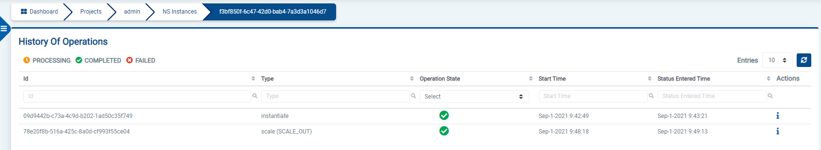
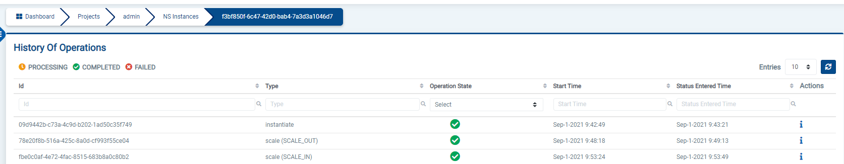
Let some minutes go by and check that a scale-out operation has been performed using the OSM GUI:
Using the K8s CLI it is possible to know exactly what the AI Agent is doing:
ubuntu@osm10:~$ kubectl get pods -n osm
NAME                                           READY   STATUS      RESTARTS   AGE
eechart-0093563749-ai-agent-1630482360-4sjwd   0/1     Completed   0          2m27s
eechart-0093563749-ai-agent-1630482420-6g44g   0/1     Completed   0          86s
eechart-0093563749-ai-agent-1630482480-pnjlw   0/1     Completed   0          26s
grafana-755979fb8c-k6xld                       2/2     Running     0          34d
kafka-0                                        1/1     Running     0          34d
keystone-786dbb778d-qk8z5                      1/1     Running     0          34d
lcm-69d8d4fb5c-kmzd7                           1/1     Running     0          34d
modeloperator-77865c54-44ddm                   1/1     Running     0          34d
mon-7c966fccfb-22zqz                           1/1     Running     0          34d
mongodb-k8s-0                                  2/2     Running     0          34d
mongodb-k8s-operator-0                         1/1     Running     0          34d
mysql-0                                        1/1     Running     0          34d
nbi-6c8b6dffb4-rjd7g                           1/1     Running     0          34d
ng-ui-6d55c58954-wq7d8                         1/1     Running     0          34d
pol-66bff9db8c-nhhl5                           1/1     Running     0          34d
prometheus-0                                   1/1     Running     0          34d
ro-5d958cc7f9-cgzrl                            1/1     Running     0          34d
zookeeper-0                                    1/1     Running     0          34d
Pendiente: ¿por qué hay tres ‘eechart’ ahora? Explicarlo porfa. Explicar también porqué hemos cogido abajo las trazas de uno de ellos y qué es lo que se ve abajo (no podemos poner las trazas y ya está)
ubuntu@osm10:~$ kubectl logs -n osm eechart-0093563749-ai-agent-1630482480-pnjlw
{"asctime": "2021-09-01 07:48:17.889", "levelname": "INFO", "name": "utils", "message": "Checking Config:\n{'executions': [{'active': False, 'monitoring': {'endpoint': 'http://192.168.137.34:4000'}, 'model': {'endpoint': 'http://192.168.137.46:8501/v1/models/CPU-forecast-model:predict'}, 'threshold': {'function_name': 'evaluator', 'logic': \"evaluator = lambda x: True if x['predictions'][0][0] >= 0.8 else False\"}}, {'active': True, 'monitoring': {'endpoint': 'http://192.168.137.34:3000'}, 'model': {'endpoint': 'http://192.168.137.46:8501/v1/models/A2-traffic-model:predict'}, 'threshold': {'function_name': 'evaluator', 'logic': \"evaluator = lambda x: False if (x['predictions'][0][0] < x['predictions'][0][1]) else True \"}}]}"}
{"asctime": "2021-09-01 07:48:17.936", "levelname": "INFO", "name": "osm_interface", "message": "VNFi info extracted from OSM: {'member-vnf-index-ref': 'VyOS Router', 'nsi_id': 'f3bf850f-6c47-42d0-bab4-7a3d3a1046d7', 'vdu-data': [{'vdu-id-ref': 'vyos-VM', 'ip-address': '192.168.137.43', 'name': 'aiagenttest-VyOS Router-vyos-VM-0'}], 'ns_name': 'aiagenttest', 'vnfs': ['648b8bb3-7f09-41ef-8a31-d632d1a90a8a'], 'project_id': '30ec57f1-4e48-43ce-a0f1-b136d66f9f67', 'scaling-group-descriptor': 'vyos-VM_vdu_autoscale'}"}
{"asctime": "2021-09-01 07:48:17.936", "levelname": "INFO", "name": "agent", "message": "OSM Data to run model evaluation: {'member-vnf-index-ref': 'VyOS Router', 'nsi_id': 'f3bf850f-6c47-42d0-bab4-7a3d3a1046d7', 'vdu-data': [{'vdu-id-ref': 'vyos-VM', 'ip-address': '192.168.137.43', 'name': 'aiagenttest-VyOS Router-vyos-VM-0'}], 'ns_name': 'aiagenttest', 'vnfs': ['648b8bb3-7f09-41ef-8a31-d632d1a90a8a'], 'project_id': '30ec57f1-4e48-43ce-a0f1-b136d66f9f67', 'scaling-group-descriptor': 'vyos-VM_vdu_autoscale'}"}
{"asctime": "2021-09-01 07:48:17.936", "levelname": "INFO", "name": "agent", "message": "Not Running {'active': False, 'monitoring': {'endpoint': 'http://192.168.137.34:4000'}, 'model': {'endpoint': 'http://192.168.137.46:8501/v1/models/CPU-forecast-model:predict'}, 'threshold': {'function_name': 'evaluator', 'logic': \"evaluator = lambda x: True if x['predictions'][0][0] >= 0.8 else False\"}} because is NOT active"}
{"asctime": "2021-09-01 07:48:17.936", "levelname": "INFO", "name": "agent", "message": "Running {'active': True, 'monitoring': {'endpoint': 'http://192.168.137.34:3000'}, 'model': {'endpoint': 'http://192.168.137.46:8501/v1/models/A2-traffic-model:predict'}, 'threshold': {'function_name': 'evaluator', 'logic': \"evaluator = lambda x: False if (x['predictions'][0][0] < x['predictions'][0][1]) else True \"}} because is active"}
{"asctime": "2021-09-01 07:48:17.936", "levelname": "INFO", "name": "agent", "message": "AI URL : http://192.168.137.46:8501/v1/models/A2-traffic-model:predict"}
{"asctime": "2021-09-01 07:48:17.936", "levelname": "INFO", "name": "model_interface", "message": "Check if AI Model Server is healthy"}
{"asctime": "2021-09-01 07:48:17.944", "levelname": "INFO", "name": "model_interface", "message": "AI Model Server reachable and up in http://192.168.137.46:8501/v1/models/A2-traffic-model:predict"}
{"asctime": "2021-09-01 07:48:18.009", "levelname": "INFO", "name": "monitoring_interface", "message": "Metrics Obtained: {'instances': [[[[0.40784314274787903, 0.529411792755127, # ..... Too long
{"asctime": "2021-09-01 07:48:18.013", "levelname": "INFO", "name": "model_interface", "message": "Preparing model request: http://192.168.137.46:8501/v1/models/A2-traffic-model:predict"}
{"asctime": "2021-09-01 07:48:18.051", "levelname": "INFO", "name": "model_interface", "message": "model requested: {'predictions': [[0.999999642, 3.18462838e-07]]}"}
{"asctime": "2021-09-01 07:48:18.051", "levelname": "INFO", "name": "threshold_interface", "message": "evaluator = lambda x: False if (x['predictions'][0][0] < x['predictions'][0][1]) else True "}
{"asctime": "2021-09-01 07:48:18.052", "levelname": "INFO", "name": "threshold_interface", "message": "Evaluating threshold: True"}
{"asctime": "2021-09-01 07:48:18.060", "levelname": "INFO", "name": "agent", "message": "SCALING OUT"}
{"asctime": "2021-09-01 07:48:18.060", "levelname": "INFO", "name": "agent", "message": "Scale kwargs {'nsi_id': 'f3bf850f-6c47-42d0-bab4-7a3d3a1046d7', 'project_id': '30ec57f1-4e48-43ce-a0f1-b136d66f9f67', 'scaling_group': 'vyos-VM_vdu_autoscale', 'vnf_index': 'VyOS Router', 'scale': 'SCALE_OUT'}"}
{"asctime": "2021-09-01 07:48:18.171", "levelname": "INFO", "name": "osm_interface", "message": "Scale action request response : {\n    \"id\": \"78e20f8b-516a-425c-8a0d-cf993f55ce04\"\n}\n"}
Accessing the ‘jam’ endpoint from a web browser, adjust again the Monitoring Service to start exposing images from the smooth traffic set (URL: http://<MonitoringServiceIP>:3000/jam)
Let some minutes go by and check that a scale-in operation has been executed.
3.2. Deploying my own AI Agent
In this section we describe how you can deploy your own AI Agents attached to your own Network Service (NS).
Step-by-step procedure
Of course, you need an OSM Release NINE (or later) installation up and running.
If you need it, you can find the installation procedure right here Install OSM based on k8s.
Develop your own AI/ML Model.
This is completely open and up to the developer to choose the technology and algorithms. Remember that as for now only models that can be used in a query-based relationship can be used (AI Agents are intended to query the AI Models hosted on the AI Models Server).
Deploy the AI Model in the AI Model Server.
The requirements to choose an AI Models Server is that it must offer an HTTP API and that it must be deployed in a network reachable from OSM. The approach is agnostic: you can use open-source implementations (e.g. TensorFlow Serving) or your own propietary solutions.
Develop the Monitoring Service.
This can be achieved in several ways as explained Monitoring Service Section.
Download the base AI Agent helm chart from the examples folder of the source repository.
The AI Agent provided can be extracted from the ai-agents_ee_vnf.tar.gz package and moved to your own VNF package directly. You can probably make yours easier from this one provided here.
Update your NS and VNF packages to ensure that they are OSM-compliant.
Refer to Descriptors section for a detailed description of the minimum parameters required to include an AI Agent.
Onboard the VNF descriptor to OSM via OSM CLI or OSM UI. Refer to OSM VNF Onboarding.
Onboard the NS descriptor to OSM via OSM CLI or OSM UI. Refer to OSM NS Onboarding.
Instantiate the NS via OSM CLI or OSM UI. Refer to OSM NS instantiation
At this point you may check the logs of the AI Agents via the K8s CLI using the following commands:
ubuntu@osm10:~$ kubectl get pods -n osm  # Locate eechart pod
ubuntu@osm10:~$ kubectl logs -n osm <eechart pod>
Service Assurance actions performed should be visible in the OSM UI
AI Agent Configuration
The deployment of the AI Agent requires the user to configure both: the descriptor that will be onboarded in OSM and the ‘values.yaml’ file from the AI Agent’s helm chart package to fully define the behavior of the agents.
The OSM descriptor configuration is available at the end of this file
The ‘values.yaml’ file contains 4 main sections which will be described here. An example can be found in Quickstart Example
Helm Chart configuration
AI Agent orchestration
For each execution:
AI Agent monitoring service configuration.
AI Agent model request for evaluation configuration.
AI Agent threshold of the model outcome configuration.
There is a full example of the ‘values.yaml’ file with two executions in Quickstart Example
Orchestration
The first part of the ‘values.yml’ is related to the AI-Agent image and the cron job execution. It allows the user to select the desired version and schedule for the execution.
jobs:
  - name: atos-ai-agent
    image:
      repository: atosresearch/osm-ai-agent
      tag: latest
      imagePullPolicy: Always
    schedule: "* * * * *"
    failedJobsHistoryLimit: 2
    successfulJobsHistoryLimit: 2
    concurrencyPolicy: Allow
    restartPolicy: OnFailure
    config:
      executions:
        # List of executions
They are all K8s standard variables defined in the official documentation.
Monitoring
The AI Agent is compatible with 2 sources of monitoring metrics to feed to the AI Model.
External: Any external source of monitoring data can be configured within values.yml to be used as data source as long as they expose a HTTP endpoint in a network known by OSM (where the EE and therefore the AI AGents will be deployed).
Internal: The deployed VDU can also be used as source of monitoring data. Since OSM will attach the ip, the user is expected to configure the corresponding monitoring section in values.yml with endpoint: vnf:<port>/<endpoint> so that the AI Agent infers that it shall request OSM for the final IP of the VDU.
This section is enclosed within each Execution item.
monitoring:
     endpoint: "http://192.168.137.34:4000"
Model
An AI Agent needs to connect to an AI Model Server that contains the desired trained model. This service must expose a HTTP endpoint in a network known by the VDU.
This section is enclosed within each Execution item.
model:
  endpoint: "http://192.168.137.46:8501/v1/models/CPU-forecast-model:predict"
Threshold
The output of the AI Model is returned back to the AI Agent where it will be evaluated using the defined threshold lambda function configured in values.yml.
This section is enclosed within each Execution entry.
threshold:
  function_name: evaluator
  logic: "evaluator = lambda x: True if x['predictions'][0][0] >= 0.8 else False"
OSM Descriptors
The provided example is found in the Source code,
Network Service
Implements a very simple deployment of the underlying VNF.
nsd:
  nsd:
  - description: Single VyOS Router VNF with AI-agents metrics
    df:
    - id: default-df
      vnf-profile:
      - id: VyOS Router
        virtual-link-connectivity:
        - constituent-cpd-id:
          - constituent-base-element-id: VyOS Router
            constituent-cpd-id: vnf-mgmt-ext
          virtual-link-profile-id: extnet
        - constituent-cpd-id:
          - constituent-base-element-id: VyOS Router
            constituent-cpd-id: vnf-internal-ext
          virtual-link-profile-id: internal
        - constituent-cpd-id:
          - constituent-base-element-id: VyOS Router
            constituent-cpd-id: vnf-external-ext
          virtual-link-profile-id: extnet
        vnfd-id: ai-agents_ee-vnf
    id: ai-agents_ee-ns
    name: ai-agents_ee-ns
    version: '1.0'
    virtual-link-desc:
    - id: extnet
      mgmt-network: true
    - id: internal
    - id: external
    vnfd-id:
    - ai-agents_ee-vnf
Virtual Network Function
Provides a single VDU configured to provide a scaling-aspect (required to trigger scaling actions) and execution-environment-list (required to link the AI Agent to the EE). You can refer to the OSM Documentation for further information.
The following example of a VNFD is extracted from the use case provided in /examples.
Notes:
Only the strictly required configuration for the AI Agent is shown here.
It includes a reactive scaling procedure which will continue to work with no differences but in this case with a proactive scaling procedure on top of it.
vnfd:
  description: A basic virtual router with AI-Agents metrics collection
  df:
  - id: default-df
    instantiation-level:
    - id: default-instantiation-level
      vdu-level:
      - number-of-instances: 1
        vdu-id: vyos-VM
    scaling-aspect:
    -   aspect-delta-details:
            deltas:
            -   id: vyos-VM_vdu_autoscale-delta
                vdu-delta:
                -   id: vyos-VM
                    number-of-instances: 1
        id: vyos-VM_vdu_autoscale
        max-scale-level: 5
        name: vyos-VM_vdu_autoscale
        scaling-policy:
        -   cooldown-time: 120
            name: vyos-VM_cpu_utilization
            scaling-criteria:
            -   name: vyos-VM_cpu_utilization
                scale-in-relational-operation: LT
                scale-in-threshold: 10
                scale-out-relational-operation: GT
                scale-out-threshold: 80
                vnf-monitoring-param-ref: vyos-VM_vnf_cpu_util
            scaling-type: automatic
    vdu-profile:
    -   id: vyos-VM
        max-number-of-instances: 6
        min-number-of-instances: 1
    vdu-profile:
    - id: vyos-VM
      min-number-of-instances: 1
    lcm-operations-configuration:
      operate-vnf-op-config:
        day1-2:
        - config-primitive:
          execution-environment-list:
          - external-connection-point-ref: vnf-mgmt-ext
            helm-chart: eechart
            id: monitor
            metric-service: ai-agent
          id: ai-agents_ee-vnf
          initial-config-primitive:
  ext-cpd:
  - id: vnf-mgmt-ext
    int-cpd:
      cpd: vdu-eth0-int
      vdu-id: vyos-VM
  - id: vnf-internal-ext
    int-cpd:
      cpd: vdu-eth1-int
      vdu-id: vyos-VM
  - id: vnf-external-ext
    int-cpd:
      cpd: vdu-eth2-int
      vdu-id: vyos-VM
  id: ai-agents_ee-vnf
  mgmt-cp: vnf-mgmt-ext
  product-name: ai-agents_ee-vnf
  sw-image-desc:
  - id: vyos-1.1.7
    image: vyos-1.1.7
    name: vyos-1.1.7
  vdu:
  - cloud-init-file: vyos-userdata
    id: vyos-VM
    int-cpd:
    - id: vdu-eth0-int
      virtual-network-interface-requirement:
      - name: vdu-eth0
        position: 0
        virtual-interface:
          type: PARAVIRT
    - id: vdu-eth1-int
      virtual-network-interface-requirement:
      - name: vdu-eth1
        position: 1
        virtual-interface:
          type: PARAVIRT
    - id: vdu-eth2-int
      virtual-network-interface-requirement:
      - name: vdu-eth2
        position: 2
        virtual-interface:
          type: PARAVIRT
    name: vyos-VM
    monitoring-parameter:
    - id: vyos-VM_vnf_cpu_util
      name: vyos-VM_vnf_cpu_util
      performance-metric: cpu_utilization
    supplemental-boot-data:
      boot-data-drive: true
    sw-image-desc: vyos-1.1.7
    virtual-compute-desc: vyos-VM-compute
    virtual-storage-desc:
    - vyos-VM-storage
  version: '1.0'
  virtual-compute-desc:
  - id: vyos-VM-compute
    virtual-cpu:
      num-virtual-cpu: 1
    virtual-memory:
      size: 2.0
  virtual-storage-desc:
  - id: vyos-VM-storage
    size-of-storage: 10